[latex]{\LARGE BAL_i(t) = G(t) \cdot (1 – p_i(t))}[/latex] with [latex]{\LARGE p_i(t) = \frac{1}{G(t)} \sum\limits_{\leq g_i(t)} g_i(t)}[/latex]
What does it mean?
The formula quantifies the sum of the basal areas of all trees that are larger or equal in basal area compared to that of a given tree i at time t. It is the complement value of the basal area percentile [latex]p_i(t)[/latex] of tree i denoting relative dominance, where G(t) is basal area per hectare of a given forest stand at time t. Basal area of an individual tree is the cross-sectional area of its stem usually measured at 1.3 m above ground level. For convenience basal area is often calculated from stem diameter using the area formula of a circle. Basal area per hectare is a density measure taking both number of trees and their sizes in a certain area into account.
BAL is related to available light, since with increasing basal area of larger trees there is less light available for smaller trees. In a sense BAL is a surrogate for light measurements with the benefit that stem diameters and basal area are easier to measure.
Where does it come from?
Basal area in larger trees is also referred to as overtopping basal area suggesting the nature of a kind of competition index. In fact this was precisely the context in which Schütz (1975), Wykoff et al. (1982) and Wykoff (1990) suggested this measure.
Why is it important?
Basal area in larger trees is a simple and effective measure that simultaneously considers relative dominance of a tree and density. It is very flexible and can easily be modified to a spatially explicit measure of competition by calculating it specifically for an influence zone around a tree. BAL is also a very suitable competition index for trees in small-sized sample plots. Naturally it is also possible to distinguish between different species and inter- and intraspecific versions of BAL. It is also easy to modify basal area in larger trees in such a way that it better explains growth rate, e.g. BAL(t)/G(t) (Wykoff, 1990). Schröder and Gadow (1999) suggested a modification which they referred to as BALMOD(t):
[latex]BALMOD_i(t) = \frac{1 – p_i(t)}{RS(t)} =\frac{BAL_i(t)/G_i(t)}{RS(t)} [/latex] with [latex]RS(t) = \frac{\sqrt{10000/N}}{H_{100}(t)}[/latex]
RS(t) is referred to as relative spacing, another density measure linking average growing space with top or dominant height, [latex]H_{100}(t)[/latex], a characteristic of growth and site quality. Top or dominant height is often calculated as the mean height of the hundred largest trees per hectare. BALMOD(t) is useful in situations where a competition index is needed for fitting a function estimating growth rates from a multiple number of different time series scattered across a certain larger geographic entity, for example a country or even a continent. In such a context, Schröder and Gadow (1999) found that BALMOD(t) is superior to BAL(t). Other authors have applied the BAL concept to crown variables and Burkhart and Tomé (2012, p. 202ff.) give a good overview.
How can it be used?
Another important purpose of the BAL concept is its use for growth analysis. Scatter plots of absolute stem-diameter growth rate, AGR(t), of the trees of a given stand for a given time, t, over BAL(t) can be depicted. Following Schütz (1975) this relationship can the be described for example by a simple power function:
[latex]AGR(t) = a + b \cdot BAL(t)^c [/latex]
a, b and c are regression coefficients. However, it is best to set c to a fixed value between 1.5 and 4. The larger the value of c the stronger the saturation effect towards the lower range of BAL and the larger the value of the growth compensation point. For comparisons within the same time series it is probably best to set c to an optimised constant value. A value of c = 2 is a good starting point.
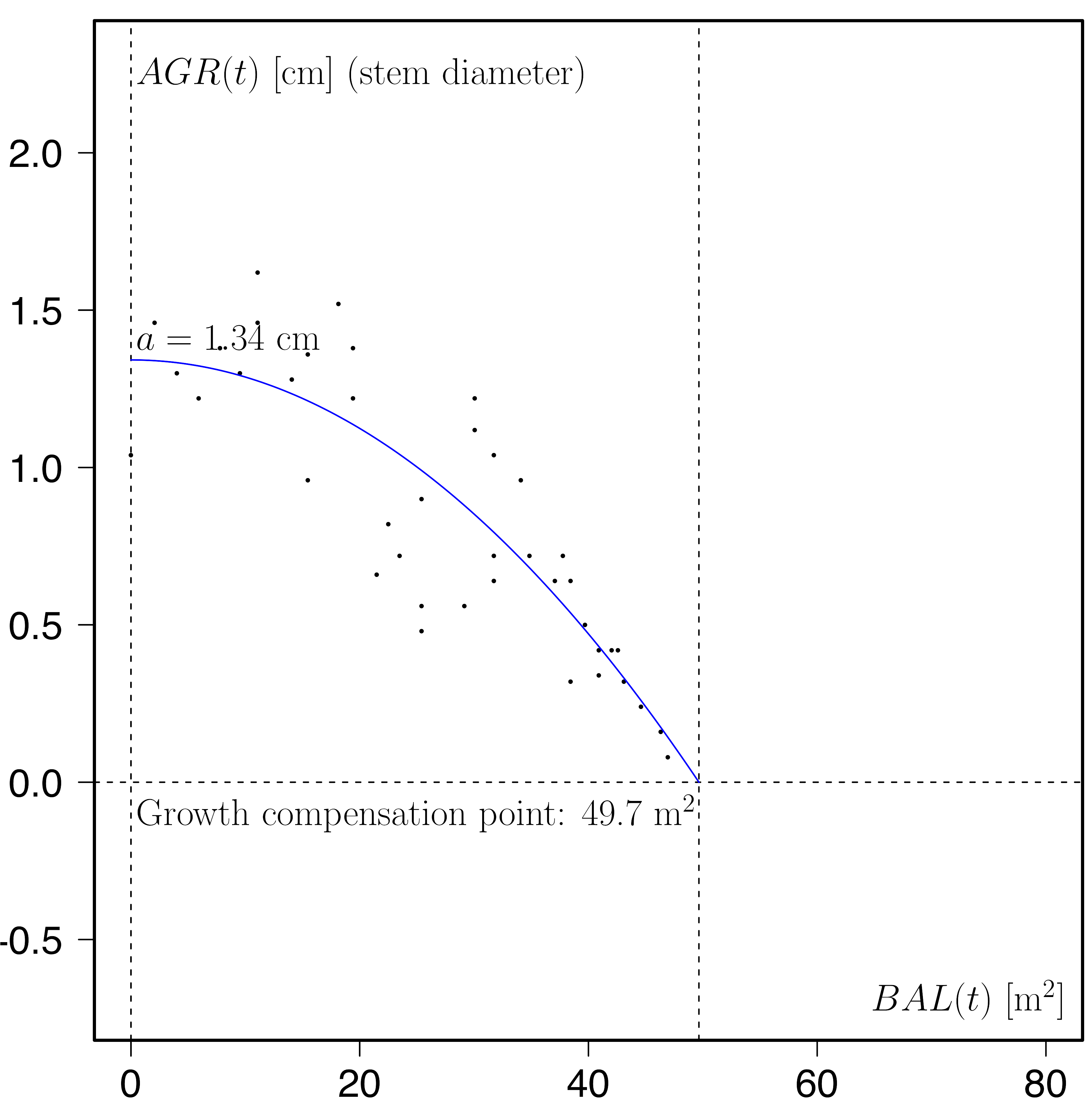
The regression coefficient a is then the intercept describing the stem-diameter growth rate of large, dominant trees (almost open-grown trees) whilst the function has a root at [latex]\sqrt[c]{a/b}[/latex]. This is the growth compensation point in analogy to the light compensation point. The growth compensation point is an expression of carrying capacity and site quality. The graph shown above is an example of this relationship for the Sitka spruce time series 2068 in the Brecon Beacons (Wales, UK, between 1961 and 1966).
Such graphs can offer valuable insights of the growth patterns of forest ecosystems in relation to density and size. Comparisons between different forest stands and tree species in the same stand (Schütz and Pommerening, 2013) are helpful in understanding the relationships between environment, size and growth. The graph below, for example, has been produced using the data from the birch-plantation time series Bagshot (England, UK). The data points represent the total time series. For fitting the saturation curves the growth data of only two subsequent survey years were used. Model parameter c was set to 2. The numbers under the dashed horizontal line give the base calendar years of the corresponding survey period.
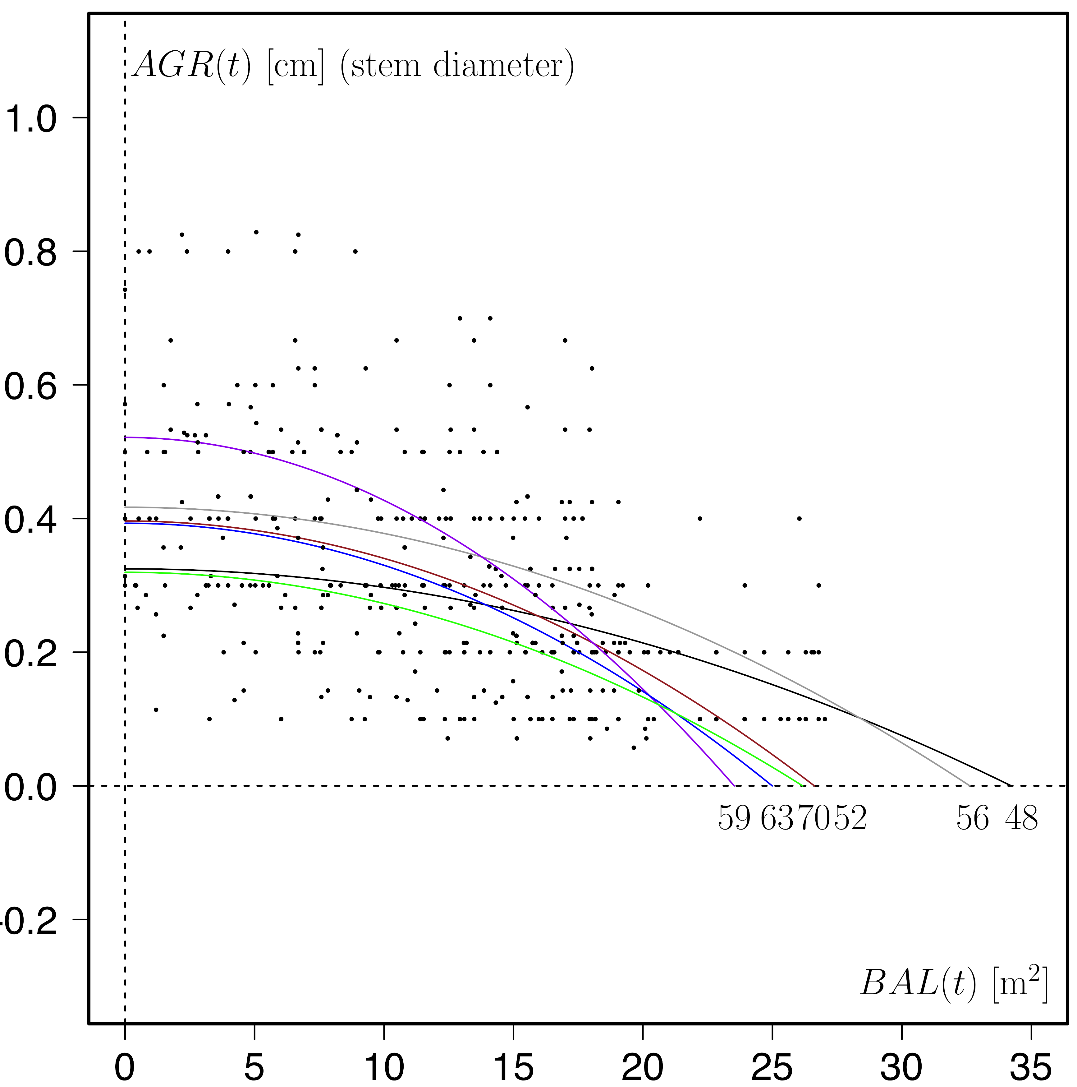
Apparently, growth compensation point and maximum growth rate (parameter a) vary throughout the years with hardly any particular pattern. Partly this can be attributed to forest management activities and partly to changing environmental conditions.
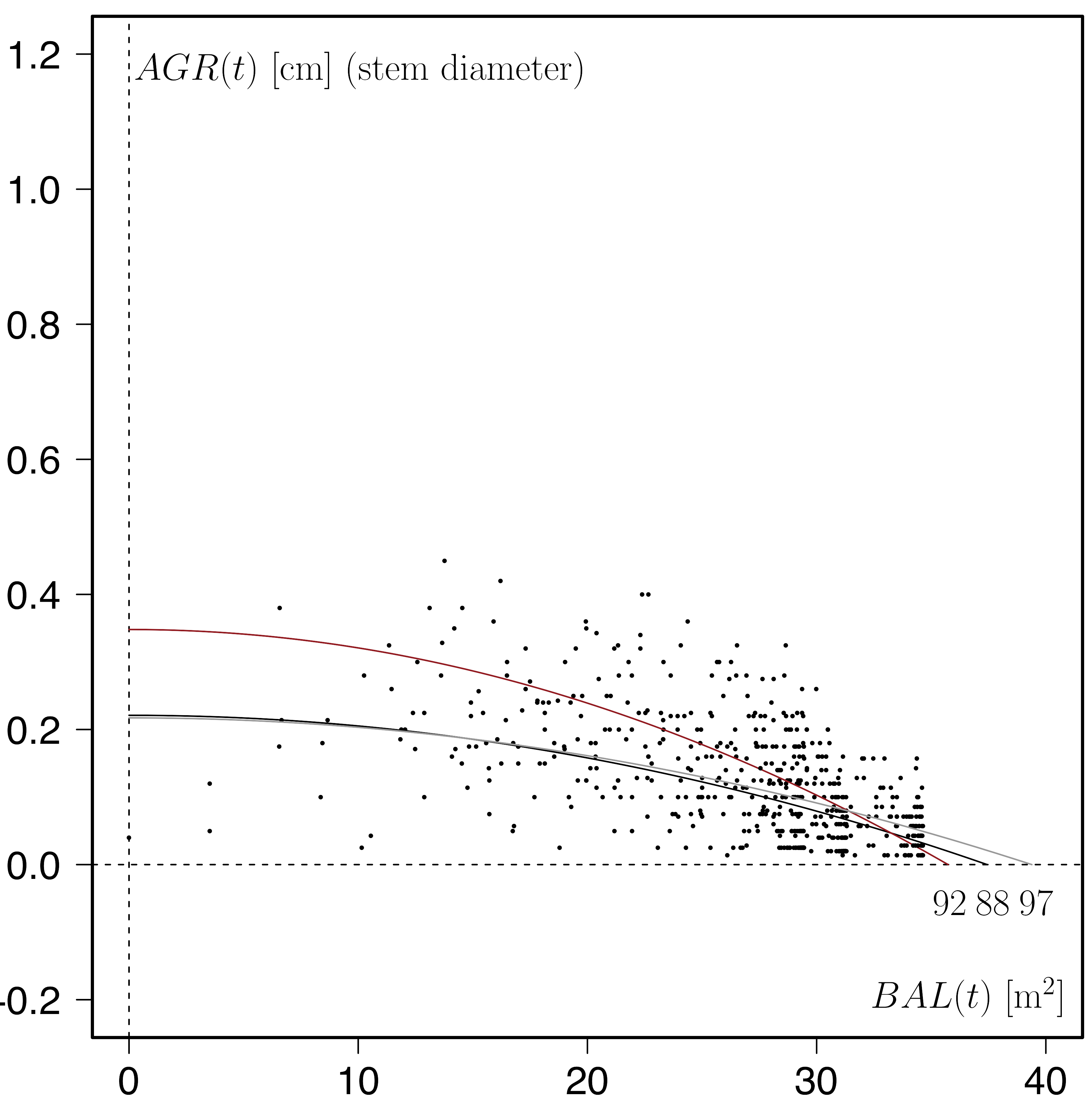
In natural, unmanaged forests, such as an Interior-Douglas fir stand in the Alex Fraser Experimental Forest (plot 3, see graph below) in British Columbia (Canada), the saturation curves and the growth compensation points are typically much closer together and show a stronger saturation effect.
Another way to illustrate and analyse the BAL – AGR relationship is to use the growth dominance characteristic that I introduced in an earlier blog in 2015.
As mentioned above, BAL(t) of an individual tree can also be used as a competition index for estimating growth rate. In that case basal area of larger trees is one of a number of explanatory variables that is either used directly in a growth function or as part of a modifier function (usually an exponential function). In the potential-modifier approach (see Weiskittel et al., 2011, p. 89ff.), first potential growth rate is estimated (e.g. growth of open-grown trees or the growth of a certain, upper percentile) and then reduced by a number of modifiers, one of which usually is competition.
R code
For calculating basal area in larger trees it is best to define a function in R that you can use at multiple instances in your R script. Such a function could look like the code given in the box below:
bal <- function(ba, area) {
 sumba <- sum(ba)
 basmaller <- 0
 pix <- 0
 bal <- 0
 for (i in 1 : length(ba)) {
   bax <- ba[i]
   basmaller <- sum(ba[ba <= bax])
   pix <- basmaller / sumba
   bal[i] <- sumba * (1 - pix) / area
 }
 return(bal)
}
Here “ba” is a vector of individual-tree basal area values and “area” is the area of the forest stand in hectare. You can then call this function in your script in the following way:
dataOneYear$ba <- pi * (dataOneYear$DBH / 200)^2
xarea <- plotSize / 10000
dataOneYear$bal <- bal(dataOneYear$ba, xarea)
“dataOneYear” is an arbitrary data frame, “dataOneYear$DBH” is a vector of stem diameters measured in cm. “plotSize” is the area of the forest stand in square metres.
Literature
Burkhart, H. and Tomé, M., 2012. Modeling forest trees and stands. Springer, Dordrecht.
Schütz, J. P., 1975. Dynamique et conditions d’équilibre de peuplements jardinés sur les stations de la hêtraie à sapin. Schweizerische Zeitschrift für Forstwesen 126: 637-671.
Schütz, J.P. and Pommerening, A., 2013. Can Douglas fir (Pseudotsuga menziesii (Mirb.) Franco) sustainbly grow in complex forest structures? Forest Ecology and Management 303: 175-183.
Schröder, J. and Gadow, K. v., 1999. Testing a new competition index for maritime pine in northwestern Spain. Canadian Journal of Forest Research 29: 280-283.
Weiskittel, A. R., Hann, D. W., Kershaw, J. A. and Vanclay, J. K., 2011. Forest growth and yield modeling. John Wiley & Sons, Chichester.
Wykoff, W. R., Crookston, N. L., Stage, A. R., 1982. User’s guide to the stand prognosis model. USDA Forest Service, Intermountain Forest an Range Experiment Station, Ogden, General Technical Report INT-133.
Wykoff, W. R., 1990. A basal area increment model for individual conifers in the northern Rocky Mountains. Forest Science 26: 1077-1104.
Dear Sir/madam
Thank you for this explanation but I have question, my question is : how can we implement BAL calculation in Netlogo ? any help or hint ?
Thank you in advance,
Tamim
You can program in Netlogo almost like with any other programming language, so the implementation should not be difficult. However, the statistical analysis needs to be done in R or similar statistical packages.
great explanation Arne!!, greetings
Dear Arne,
is there a refrence, ie. an article, to cite the content of this blog?
I thank you.
Dear Chiara,
There hasn’t been published much on this subject. You can check out Schütz and Pommerening (2013) on http://www.pommerening.org. Still a lot of potential to work on.
/Arne
No, this hasn’t been published yet. There is a little bit about this in Schütz and Pommerening (2013), see my reference list on pommerening.org.