[latex]M_i^{(k)} = \frac{1}{k}\sum_{j = 1}^k \textbf{1}(species_i \ne species_j)[/latex]
j denotes the jth nearest neighbour of plant i. The expression 1(A) = 1, if condition A is true, otherwise 1(A) = 0. In principle, k can take any number and can also vary between plants of the same population or research plot. However, for convenience k has often been set to a fixed value of 3 or 4, but this convenience lacks scientific justification.
What does it mean?
The mingling index [latex]M_i^{(k)}[/latex] is defined as the mean fraction of plants among the k nearest neighbours of a given plant i with heterospecific neighbours.
Where does it come from?
An early strategy and benchmark for quantifying spatial species mingling is Pielou’s segregation index (Pielou, 1977) comparing pairs of points formed by the locations of an arbitrary plant and its nearest neighbour. For all plants in a certain observation window (e.g. a research plot) these pairs are determined. Pielou (1977) defined the segregation index as the ratio of the observed probability that an arbitrary plant and its first nearest neighbour are conspecific and the same probability with independent species marks (i.e. a completely random dispersal of species). This segregation index was originally developed for bivariate species patterns and describes the neighbourhood structure of a subject plant of one species in terms of others. An individual has a high degree of mingling if its neighbourhood is highly diverse, i.e. if many heterospecific neighbours are located in its vicinity. The opposite of a largely conspecific neighbourhood is referred to as segregation.
Gadow (1993) and Aguirre et al. (2003) extended this concept to general multivariate species patterns involving k neighbours.
Why is it important?
Species diversity is an important and most commonly considered aspect of biodiversity worldwide (Kimmins, 2004). As a part of species diversity, spatial mingling of plants concerns the question of how plants of the same and different species mix in space. This refined concept extends beyond the idea of species richness to take the individuals’ perception of local diversity into account. Spatial mingling specifically relates to the microstructure of ecosystems, particularly to neighbourhood relationships, which play a vital role in plant ecology.
How can it be used?
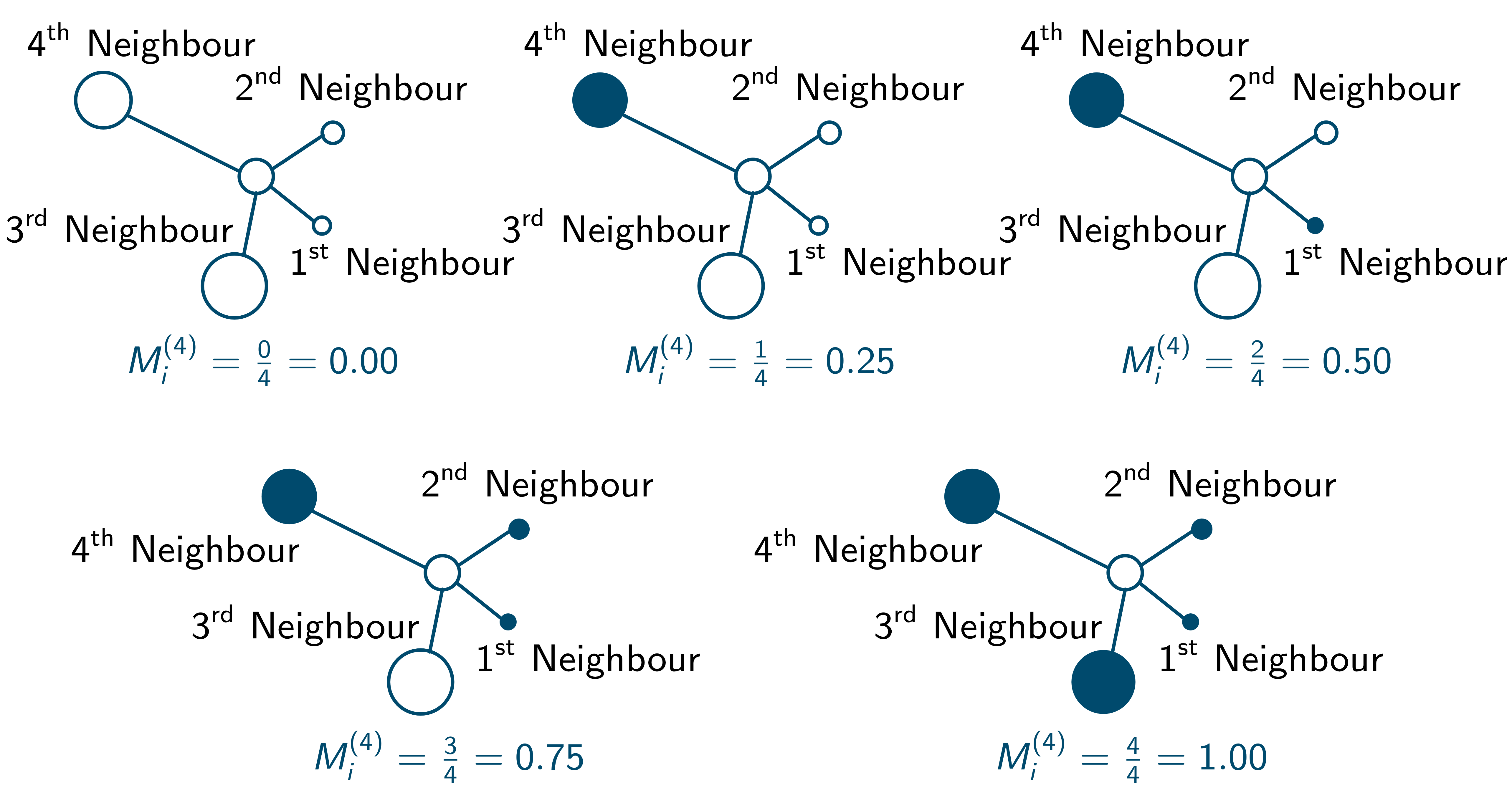
With k number of neighbours the mingling index [latex]M_i^{(k)}[/latex] can take k + 1 different discrete values depending on the neighbourhood situation. This is illustrated for k = 4 in the following illustration, where the colours of the circular plant objects represent different species:
These discrete mingling values can be used to construct an empirical mingling distribution, which collects the relative numbers of plants with one of the k + 1 [latex]M^{(k)}[/latex] values and presents them as bars.
It is also possible to estimate arithmetic mean mingling, [latex]\overline{M}^{(k)}[/latex], at population level using an appropriate edge correction method such as NN1 (Pommerening and Stoyan, 2006).
Empirical mingling distributions and mean arithmetic mingling can also be calculated separately for individual species populations of the same plant population.
According to Lewandowski and Pommerening (1997) expected mingling (implying independent species marks), EM, is independent of the number of nearest neighbours, k, and can be calculated as
[latex]\textbf{E}M = \sum_{i = 1}^s \frac{N_i (N – N_i)}{N (N – 1)}[/latex]
with s, the number of species, N, the total number of plants in the observation window and [latex]N_i[/latex], the number of plants of species i.
In analogy to Pielou’s segregation index [latex]\overline{M}^{(k)}[/latex] and EM can be arranged in an index M expressing the relationship between observed species mingling and completely random species mingling according to
[latex]M = 1 – \frac{\overline{M}^{(k)}}{\textbf{E}M}[/latex].
I refer to this index as species segregation index. Consequently, M = 0 if the species marks are independent or random. If the nearest neighbours and plant i always share the same species, M = 1 (attraction of similar species, segregation in Pielou’s terminology). If all neighbours always have a species different from that of plant i, M = -1 (attraction of different species, aggregation in Pielou’s terminology).
R code
To calculate M two auxiliary functions are necessary, the first one calculating EM and the second one calculating the Euclidean distance.
calcExpectedMinglingAllSpecies <- function(species) {
  ta <- table(species)
  s <- length(ta)
  ka <- length(species)
  swm <- 0
  for (i in 1 : s)
    swm <- swm + ta[[i]] * (ka - ta[[i]]) / (ka * (ka - 1))
  return(swm)
}

euclid <- function(x1, y1, x2, y2) {
  dx <- abs(x2 - x1)
  dy <- abs(y2 - y1)
  dz <- dx^2 + dy^2
  return(dz^0.5)
}
The main calculations are done in the following loop and additional lines of code. Here the NN1 edge correction is used for estimating arithmetic mean mingling.
myData$sming <- NA
myData$dist <- NA
myData$rf <- NA

k <- 4
for (i in 1 : length(myData$x)) {
 sums <- 0
 dn <- findNeighboursOfOnePoint(myData$x, myData$y, k, i)
 for (j in 1 : k) {
   index <- dn[j] + 1 # Correcting C++ indices
   if(myData$species[i] != myData$species[index])
     sums <- sums + 1
   if(j == k) {
     dist <- euclid(myData$x[i], myData$y[i], myData$x[index],
             myData$y[index])
     myData$dist[i] <- dist
     myData$rf[i] <- calcRepFactor(xmax, ymax, myData$x[i], myData$y[i],
                     dist)
   }
 }
 myData$sming[i] <- sums / k
}

sums <- sum(myData$sming * myData$rf)
sumRF <- sum(myData$rf)
(mm <- sums / sumRF)
(em <- calcExpectedMinglingAllSpecies(myData$species))
(m <- 1 - mm / em)
“xmax” and “ymax” define the boundary of the observation window whose bottom left corner coincides with the origin of the system of coordinates. The functions “findNeighboursOfOnePoint” and “calcRepFactor” are implemented in external C++ files that can be made available on request and are loaded in the following way:
library(Rcpp)
sourceCpp(paste(filePath, "findNeighboursOfOnePoint.cpp", sep = ""))
sourceCpp(paste(filePath, "NN1.cpp", sep = ""))
Literature
Aguirre, O., Hui, G. Y., Gadow, K. and Jiménez, J., 2003. An analysis of spatial forest structure using neighbourhood-based variables. Forest Ecology and Management 183: 137-145.
Gadow, K. v., 1993. Zur Bestandesbeschreibung in der Forsteinrichtung. [New variables for describing stands of trees.] Forst und Holz 48: 602-606.
Kimmins, J. P., 2004. Forest ecology. A Foundation for sustainable forest management and environmental ethics in forestry. 3rd edition. Pearson Education, Inc., Upper Saddle River.
Lewandowski, A. and Pommerening, A., 1997. Zur Beschreibung der Waldstruktur – Erwartete und beobachtete Arten-Durchmischung. [On the description of forest structure – Expected and observed mingling of species.] Forstwissenschaftliches Centralblatt 116: 129-139.
Pielou, E. C., 1977. Mathematical ecology. John Wiley & Sons, New York.
Pommerening, A. and Stoyan, D., 2006. Edge-correction needs in estimating indices of spatial forest structure. Canadian Journal of Forest Research 36: 1723-1739.