The Weibull density distribution is known as
[latex]f_w(dbh) = \frac{\gamma}{\beta}\left(\frac{dbh – \alpha}{\beta}\right)^{\gamma – 1} e^{-\left(\frac{dbh – \alpha}{\beta}\right)^\gamma}[/latex],
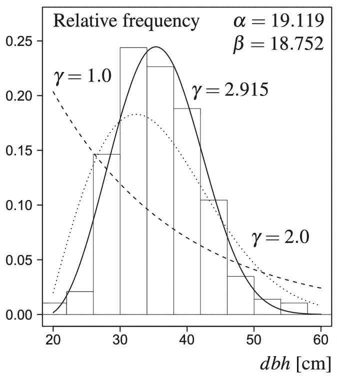
where [latex]\alpha[/latex] is the location, [latex]\beta[/latex] the scale and [latex]\gamma[/latex] is the shape parameter, i.e. the parameters of the Weibull distribution are interpretable, which is always a good property of models.
The cumulative distribution function, i.e. the integral of density function, is much simpler:
[latex]F_w(dbh) = 1 – e^{\left(\frac{dbh – \alpha}{\beta}\right)^{\gamma}}[/latex]
What does it mean?
The Weibull density distribution allows characterising tree stem-diameter distributions by providing trend curves but more importantly by summarising stem diameters by means of three parameters that can be interpreted.
The shape parameter of the Weibull distribution, [latex]\gamma[/latex] is of particular interest in this context and the following interpretation aid can be used (Burkhart and Tomé, 2012, p. 198):
When [latex]\gamma[/latex] is less than 1, the distribution is reverse j-shaped found in uneven-aged forest stands and when [latex]\gamma[/latex] equals 1, a negative exponential distribution results. If [latex]\gamma = 3.6[/latex], the Weibull distribution approximates a normal distribution and this value divides left- and right-skewed curves. In general, [latex]\gamma > 1[/latex] gives bell-shapes typical of even-aged forest stands. The location parameter is directly related to the minimum diameter in a stand (Burkhart and Tomé, 2012, p. 265 ). In the context of diameter distributions, all model parameters must be positive.
Where does it come from?
The Weibull distribution is named after Swedish mathematician Waloddi Weibull, who described it in detail in 1951, although it was first identified by Fréchet (1927) and first applied by Rosin and Rammler (1933) to describe a particle size distribution.
Why is it important?
The Weibull distribution is one of the most flexible and most commonly applied model for tree stem-diameters. The model parameters are comparatively easy to estimate and the distribution is easy to apply.
How can it be estimated?
Robinson and Hamann (2010, p. 164ff.) described in detail how the three parameters of the Weibull distribution can be estimated using R and the maximum-likelihood method. The grey box below gives an adaptation of that method:
dweibull3 <- function(x, gamma, beta, alpha) {
   (gamma/beta) * ((x -alpha)/beta)^(gamma - 1) * (exp(-((x - alpha)/beta)^gamma))
 }

loss.w3 <- function(p, data)
   sum(log(dweibull3(data, p[1], p[2], p[3])))

mle.w3.nm <- optim(c(gamma = 1, beta = 5, alpha = 10),
                    loss.w3, data = myData$dbh, hessian = TRUE,
                    control = list(fnscale = -1))

mle.w3.nm$par # model parameters

# Check whether the curve looks OK
xx <- seq(10, 60, 1)
hist(myData$dbh, freq = F, breaks = 50, xlim = c(10, 60))
lines(xx, dweibull3(xx, mle.w3.nm$par[1], mle.w3.nm$par[2],
mle.w3.nm$par[3]), lty = 1, col = "red")
Since R only provides implementations for the two-parameter version, the code starts with a new function dweibull3() implementing the three-parameter version. This is followed by a maximum-likelihood loss function using the previously defined function dweibull3(). This loss function in turn now forms one of the arguments of the optim() function used for carrying out the regression. myData is a data frame that includes a vector of stem diameters that can be addressed by myData$dbh.
An alternative to nonlinear maximum-likelihood based regression are percentile estimations. The idea of this approach is to estimate the three parameters of the Weibull distribution from selected points of the distribution, e.g. the 63rd or 95th percentile. The theory of percentile estimators is well explained in Clutter et al. (1983, p. 127ff.). However, percentile estimations can be very valuable where maximum-likelihood regression does not produce any or unsuitable results. Some methods of percentile estimation have also been linked to straightforward sampling methods, so that the parameters of the Weibull function can almost be directly sampled in the field without much effort. Also, percentile methods can be used to identify starting values for nonlinear regression. Below one example method of percentile estimations is provided.
According to Wenk et al. (1990, p. 198f.) and Burkhart and Tomé (2012, p. 265)
[latex]\hat{\beta} = d_{63\%} – d_{min}[/latex].
[latex]d_{63\%} = \alpha + \beta[/latex] and can be interpreted as the diameter where approximately 63% of all trees are smaller in diameter. [latex]d_{min} = \hat{\alpha}[/latex] , i.e. the minimum diameter in a tree population or forest stand.
Finally, Gerold(1988) suggested that [latex]\gamma [/latex] can be estimated from [latex]d_{\min}[/latex] and the diameter where approximately 95\% of all trees are smaller in diameter.
[latex]\hat{\gamma} = \frac{ln(-ln(1-0.95))}{ln \left(\frac{d_{95\%}-d_{\min}}{d_{63\%}-d_{\min}}\right)} = \frac{1.09719}{ln \left(\frac{d_{95\%}-d_{\min}}{d_{63\%}-d_{\min}}\right)}[/latex]
[latex]d_{\min}[/latex], [latex]d_{63\%}[/latex] and [latex]d_{95\%}[/latex] can be estimated from any empirical diameter distribution but also by employing a simple sampling procedure. Based on a systematic sampling grid approximately ten sample points need to be identified in every forest stand along with the first twelve tree neighbours nearest to each sample point. Römisch (1983) found that [latex]d_{63\%} [/latex] can be estimated from the diameter of the fifth largest tree out of twelve sample trees and that [latex]d_{95\%}[/latex] can be estimated from the largest diameter tree out of ten sample trees nearest to the sample point. [latex]d_{63\%}[/latex] and [latex]d_{95\%}[/latex] are then calculated as the arithmetic means of all ten samples. [latex]d_{\min}[/latex] is the smallest diameter of all sample trees (Gerold, 1988).
Literature
Burkhart, H. and Tomé, M., 2012. Modeling forest trees and stands. Springer, Dordrecht.
Clutter, J. L, Fortson, J. C., Pienaar, L. V., Brister, G. H. and Bailey, R. L., 1983. Timber management. A quantitative approach. John Wiley & Sons, New York.
Fréchet, M., 1927. Sur la loi de probabilité de l’écart maximum. Annales de la Société Polonaise de Mathematique 6: 93-116.
Gerold, D., 1988. Describing stem diameter structure and its development by using the Weibull distribution. Wissenschaftliche Zeitschrift der Technischen Universität Dresden 37: 221-224.
Rosin, P. and Rammler, E., 1933. The laws governing the fineness of powdered Coal. Journal of the Institute of Fuel 7: 29–36.
Robinson , A. P. and Hamann , J. D., 2010. Forest analytics with R. An introduction. Use R! Springer. New York, 339p.
Römisch, K., 1983. A mathematical model for simulating growth and thinnings of even-aged pure stands. PhD thesis Technical University Dresden. Dresden, 197p.
Wenk, G., Antanaitis, V. and Šmelko, Š ., 1990. Forest growth and yield science. Deutscher Landwirtschaftsverlag. Berlin, 448p.
Weibull, W., 1951. A statistical distribution function of wide application. Journal of Applied Mechanics 18: 293–297.
Hej, I tried this code on my dataset, but had this error, which I have no idea how to fix:
> dweibull3
> loss.w3
> mle.w3.nm <- optim(c(gamma = 1, beta = 5, alpha = 10),
+ loss.w3, data = p4$dia, hessian = TRUE,
+ control = list(fnscale = -1))
Error in fn(par, …) : unused argument (data = p4$dia)
dweibull3 <- function(x, gamma, beta, alpha) {
(gamma/beta) * ((x -alpha)/beta)^(gamma – 1) * (exp(-((x – alpha)/beta)^gamma))
}
loss.w3 <- function(dia, p3)
sum(log(dweibull3(data, p[1], p[2], p[3])))
mle.w3.nm <- optim(c(gamma = 1, beta = 5, alpha = 10),
loss.w3, data = p4$dia, hessian = TRUE,
control = list(fnscale = -1))
Goodwin (2021) shows that the optimum (lower) bound (location parameter “a”) of the Weibull is not “directly” associated with the smallest diameter (D1), but rather, can be estimated as a function of D1, mean diameter (D), sample size N, and skewness or shape parameter (c) such that a=D1-(D-D1)/(N^(1/c)-1), where the shape parameter “c” is solely a function of skewness.
Consequently, the optimum location parameter “a” can be negative when skewness is negative, and the loss of fit suffered by constraining a>=0 in such situations can be surprisingly large – the Kolmogorov-Smirnov score can be 50% larger.
I call this phenomenon “constraint shock” because it is a large effect that will come as a surprise to forest biometricians.
The problem can be resolved with left hand truncation – but this is of course more complicated, but it is a lot more accurate than the standard approach.
There hasn’t been much work on trends in diameter skewness. Most Australian plantations are negatively skewed until around age 20 or until first thinning. However, before assuming that a Weibull PDF with a positive bound is a good model, it’s a good idea to test for negative skewness.
Goodwin A N (2021) A Blind Spot in the Use of the Weibull Function for Modeling Diameter Distributions. For. Sci. 67(2):125-132