A summary statistic that crossed my path a lot this year is growth dominance. Growth dominance is a concentration measure based on the Lorenz curve and was invented by Dan Binkley and his lab at Colorado State University, USA. Together we have worked with this characteristic this year and it has been great fun. We applied it to data from a virgin forest and learned a lot more about growth processes in such forest types.
Growth dominance characterises the contributions of different tree sizes to total population growth (Binkley et al., 2006). West (2014) provides a good statistical description of the growth dominance concept in Forest Science.
The growth dominance curve is related to different development phases of forest stands. Young, middle-aged and old stands have characteristic curves and the statistic is therefore a useful indicator. In the context of continuous cover forestry, it is likely that growth dominance can prove a useful characteristic for quantifying the progress of transforming tree plantations to uneven-aged forests.
In this “Christmas blog”, I would like to share a simple R script for the calculation of this statistic. Reading and using it is also a good way of understanding how the growth dominance statistic works. The blog is intended for readers with a basic understanding of R and unknown bits of syntax can easily be tracked down in the internet. Here are the first three code chunks:
# Load data
dFile <- paste(filePath, "Clog1.txt", sep = "")
xdata <- read.table(dFile, header = TRUE)
# Creating the size and growth rate vector
d <- xdata$d2002
g <- pi * (d/200)^2
ig <- pi * (xdata$d2007/200)^2 - g
rm(xdata)
ig <- ig / 5
# Merging size and growth rate vector in a data frame
xdata <- data.frame(g, ig)
The first two-three chunks of code are almost self-explanatory: Data is loaded including two columns with a size variable measured at two different points in time. In this case it is stem diameter (at 1.3 m above ground level) measured in centimetres both in 2002 and 2007. The stem diameters are converted to basal areas (cross-sectional areas) and the mean annual basal-area (absolute) growth rate is calculated. Finally size vector (here initial basal area in 2002) and growth-rate vector are merged in one data frame.
The next step is important and is key to the interpretation of the growth dominance statistic. The whole data frame is ordered according to size from small to large trees, so that the size and the growth rate vectors contain corresponding pairs of values.
xdata <- xdata[order(xdata$g, decreasing = FALSE), ]
Now we calculate cumulative relative tree sizes and cumulative relative growth rates:
cumG <- cumsum(xdata$g) / sum(xdata$g)
cumInc <- cumsum(xdata$ig) / sum(xdata$ig)
Based on the cumulative vectors we can now estimate a characteristic similar to the Gini coefficient of the Lorenz curve.
area <- 0
for(i in 2 : length(cumG))
 area[i] <- (cumG[i] - cumG[i - 1]) * ((cumInc[i] - cumInc[i - 1]) /
 + 2 + cumInc[i - 1])
gc <- 1 - sum(area) / 0.5
cumInc can now be plotted over cumG to give the growth dominance curve. To obtain smooth curves, it is, however, advisable to calculate percentiles corresponding to selected points on the size axis:
x.values <- seq(0, 1, by = 0.05)
rx <- ecdf(cumG) (x.values)
sx <- quantile(cumInc, rx)
To obtain smooth curves, sx is plotted over x.values. The figure below gives an impression of the data from a roughly 55-year old Sitka spruce plantation in transformation to Continuous Cover Forestry.
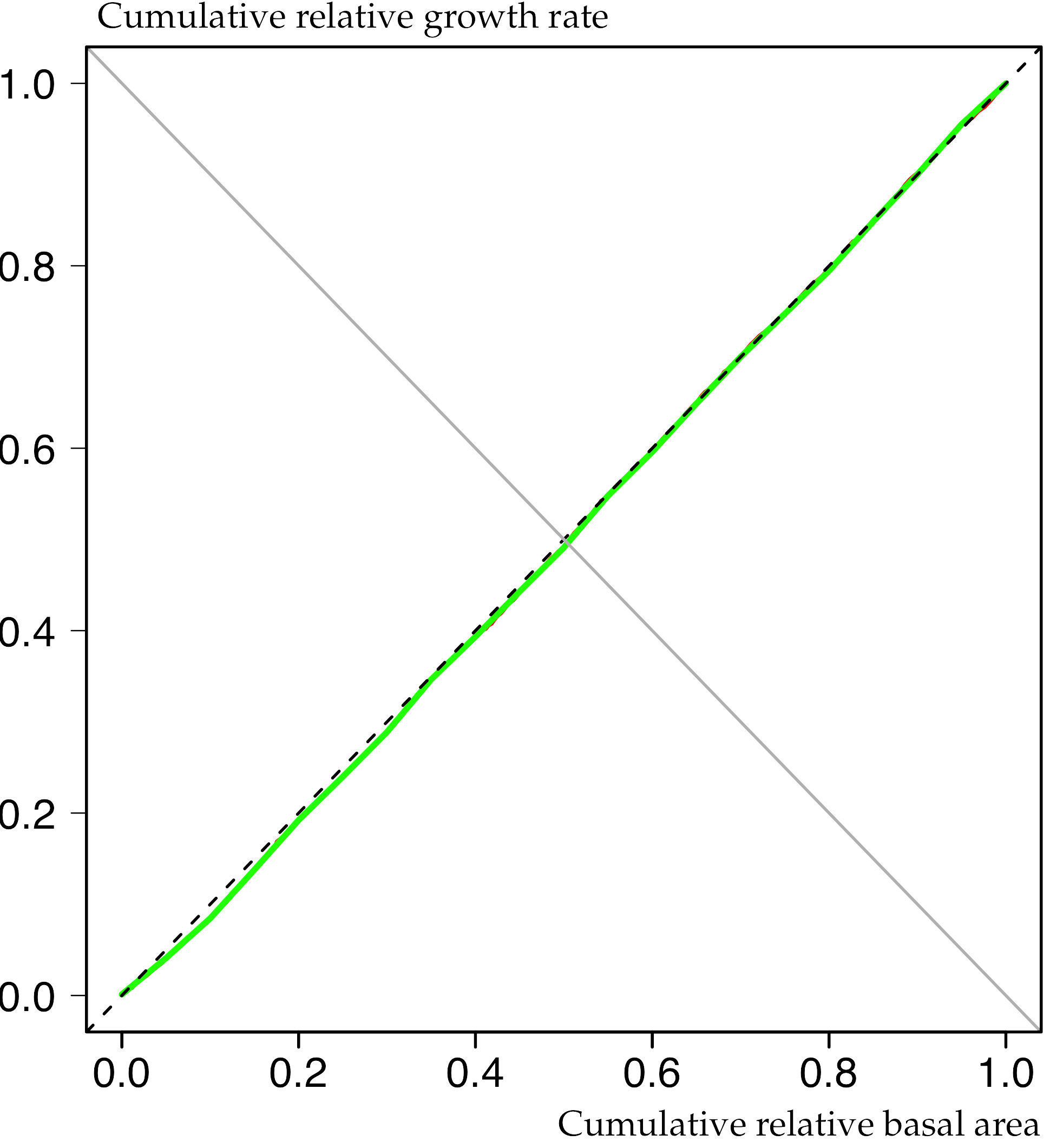
Apparently the observed growth dominance curve (continuous green line) is almost symmetric and very close to the 1: 1 (dashed) line. This is indicative of development phase 1, where each tree’s contribution to total stand growth is proportional to its size. Usually this pattern can be found in young stands before canopy closure but apparently it is also true for middle-aged plantations at the beginning of transformation.
Got intrigued? I find growth dominance quite fascinating and for me it is definitely my personal growth characteristic of the year 2015. Perhaps you would like to try this characteristic with your own data. (I can send you the full version of my R script and the data on request.) Have fun and … Merry Christmas and a Happy New Year!